

S1E5: “Proof for a case where discounting advances the doomsday”
Discounting in 1970s energy models

This post is part of a series on the history of how economists model the future with the Ramsey formula, based on joint work with Pedro Garcia Duarte. See episode 1 , episode 2, episode 3, episode 4. Full Paper here
The 1972 publication of the Meadows report, followed by the October 1973 OAPEC oil embargo, threw world citizens, governments, and economists into disarray. Based on system dynamic modelling techniques developed by MIT engineer Jay Forrester, the simulations commissioned by the Club or Rome predicted that by 2050, growing population, pollution, and overconsumption of exhaustible resources, would lead to overshoot and collapse. Combined with books like Paul Ehrlich’s The Population Bomb, this created a growing sense of uncertainty about the future.
Existing national and international organizations commissioned scenarios on world energy, economic and social futures: the International Labor Organization, the OECD and the UN produced reports entitled Catastrophe or New Society or The Future of the World Economy. In 1972, the International Institute for Applied Systems Analysis (IIASA) was established in a castle near Vienna, to foster scientific cooperation between East and West. Its large-scale interdisciplinary “Energy Project” involved more than 250 scientists, who produce a set of integrated models (MEDEE- MESSAGE-IMPACT-MACRO ) and scenarios published in 1981 as Energy in a Finite World. While France’s Messmer plan ushered the country into an era of nuclear investment, the president of the newly founded US Energy Research and Development Administration asked an ad-hoc committee, the Committee on Nuclear and Alternative Energy Systems (CONAES) to prepare an extensive study on energy mix alternatives for the coming decades.
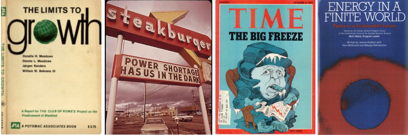
All this made economists feverish. The Meadows report had set a standard for growth and energy modeling – computational models that aimed to integrate natural and economic dynamics, all without even nodding to economists’ growth models. The efforts of the Meadows group, coupled with the energy crisis, redirected discussions around the role of exhaustible resources in growth models. In seminars, special issues and AEA lectures, these economists highligthed the flaws of what they called “doomsday models”: the lack of economic reasoning, of notions such as prices, substitution between production factors, or technological progress allowing productivity gain.
The (re)introduction of exhaustible natural resources in growth models drew economists’ attention to Harold Hotelling’s earlier result. The idea that the net price of exhaustible resources should rise at the interest rate was therefore christened the “Hotelling rule” by Bob Solow – selling the resource and reinvesting the proceed at some interest rate should be equivalent to keeping the resource and selling it at a later date. This raised the stakes for adequately determining the discount rate: it was now crucial for cost-benefit analysis, growth paths and the depletion rate of exhaustible resources.
Yet among the three landmark 1974 articles proposing growth models with exhaustible growth, Solow’s model opted for no-discounting (a decision I’ll cover in the next post). UK-based economists Partha Dasgupta and Geoffrey Heal explored a “cake eating” situation (with uncertain prospect of developing new technologies), so they choose a Ramsey model and derived a “familiar Ramsey condition” on the optimal growth path. In a 1979 book expanding on the topic, they called the equation linking the social rate of return on investment with the pure of time preference and the growth*elasticity parameter the “Ramsey rule.” “Its virtue lies in its simplicity,” they explained. “The condition brings out in the simplest manner possible the various considerations that may appear to being morally relevant in deciding the optimum rate of accumulation.”
More than these theoretical exercises, the race to build empirical energy models to study the consequences of resources and technology availability, as well as alternative energy policies, shaped debates on discounting and the circulation of the Ramsey formula. Energy modeling in the 1970s was akin to the Wild West: beyond the growing use of simulation and the need to better integrate energy supply -typically modeled by engineers - and demand -economists’ domain-, there were no established rules. Terms like Integrated Assessment Model, or top-down vs bottom-up were not yet in use. Up to the 1970s, the demand for energy was considered stable and determined by growth, with the primary objective being to minimize the costs of energy supply. The oil shock prompted economists to model the reverse linkage between the energy sector and the rest of the economy, either through partial or general equilibrium models. Estimating price elasticities, and elasticities of substitutions for various energy sources was crucial. The proliferation of models was such that in 1976, the US Energy Modeling Forum was established to compare them and facilitate closer collaboration between modelers and users.
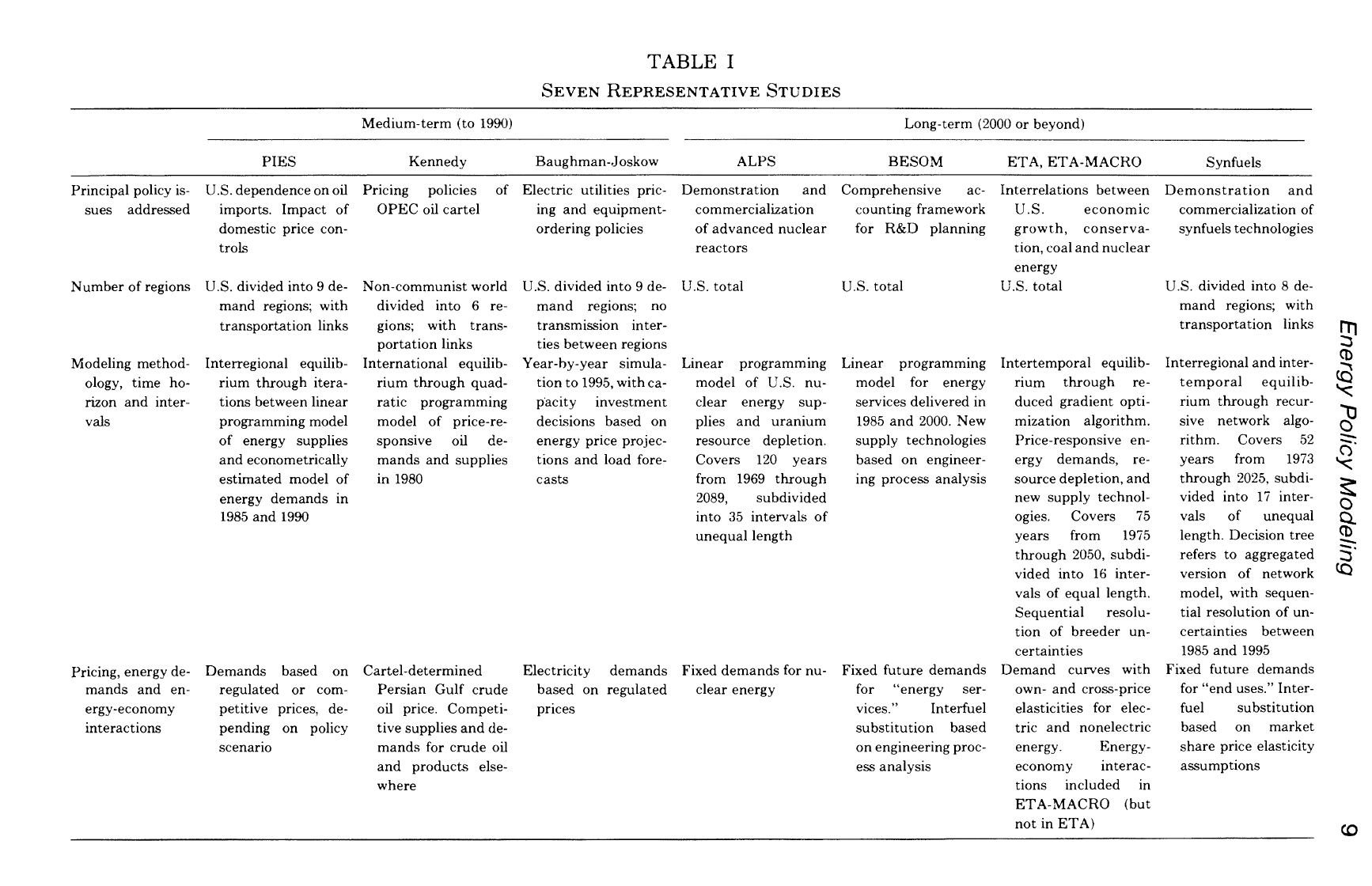
Economists’ reliance on cost-benefit analysis aligned well with governments’ needs to evaluate a range of alternative policy measures, from conservation policies to nuclear technologies investments, taxes, quotas, energy efficiency standards or utility regulation. They were thus in demand in the many institutions developing models and scenarios. In 1975, the CONAES set up a Modeling Resource Group, chaired by Koopmans, to investigate the cost and benefits of various energy options. The group employed a diverse set of models: supply-side models like DESOM or SRI; demand-side models (DRI), and three integrated equilibrium models: the PIES of William Hogan, David Nissen and James Sweeny, as well two aggregative models that maximized the sum of discounted future utilities through linear programming techniques. ETA (Energy Technology Assessment) was developed by Alan Manne and his student Richard Richels, and the other model was proposed by William Nordhaus. Just like Koopmans, both Manne and Nordhaus had just spent time at IIASA, where they refined their views of discounting.

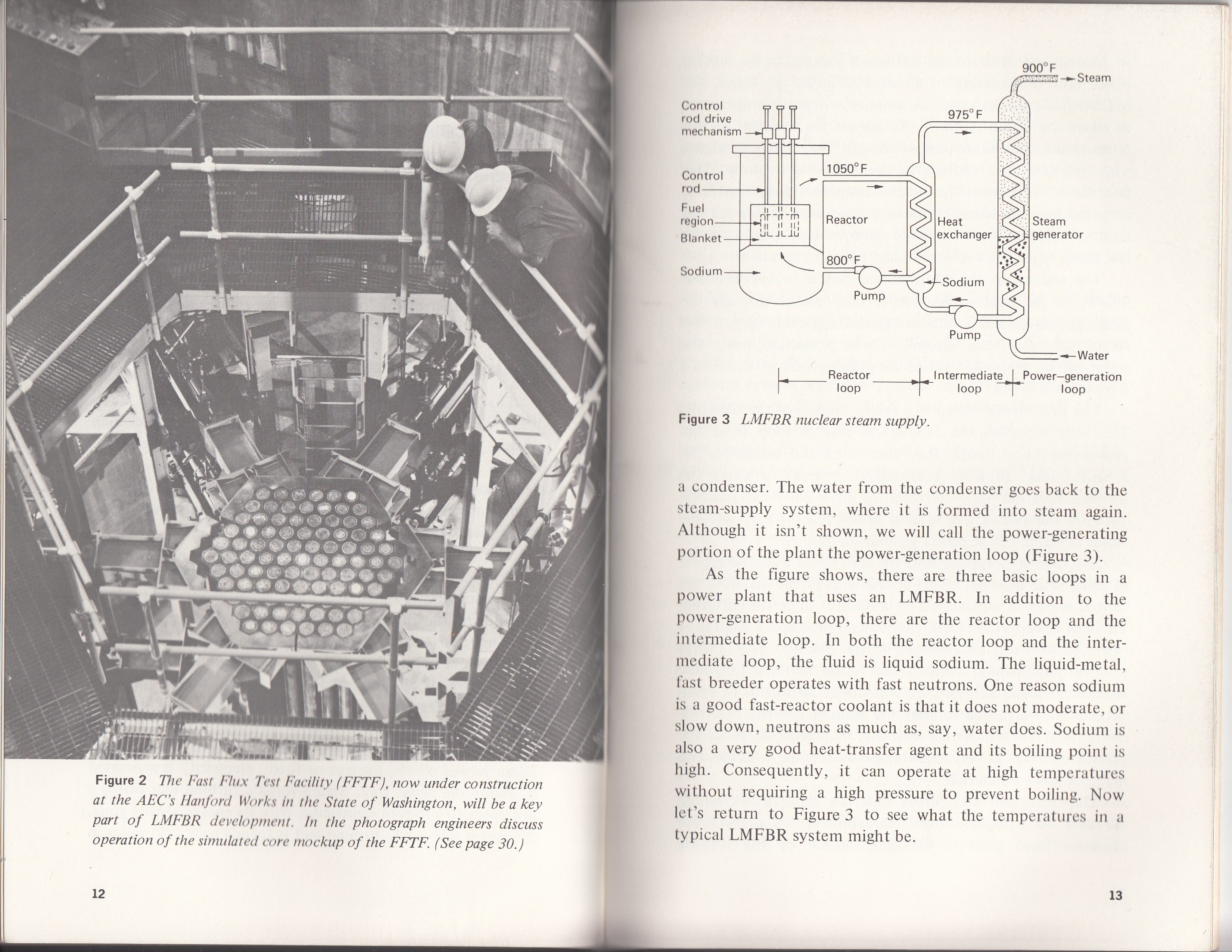
After being involved in optimal growth debates, Koopmans had continued to explore these issues. During his time at IIASA, he issued a short paper entitled “Proof for a case where discounting advances the doomsday” which examined an optimal growth model with exhaustible resources. A former RAND alumnus, Manne was then working at both the Stanford business school and Operation research Department. A specialist of OR and industrial planning, he had developed a keen interest in the energy sector, computer programming and simulation. Nordhaus later described him as the “analyst and algorithmist” of the IIASA group. At a time when American society, the government and the CONAES were deeply divided over nuclear energy, Manne used his IIASA time to focus on the breeder reactor. A new type of reactor that produced more fissile material than it consumed, it was then seen as a potential solution to the perceived scarcity of uranium (in the end, it proved more costly than water-cooler reactors and interest waned as new reserves and cheaper uranium enrichment technologies emerged).

He wrote a paper investigating which combination of energy sources should be used while “Waiting for the Breeder.” It employed sequential probabilistic linear programming (decisions trees). His findings revealed that a 10% discount rate made near future decisions insensitive to the long term technological uncertainty, whereas a 3% rate significantly enhanced the appeal of nuclear power over fossil fuel. Manne detailed potential objections to lowering the discount rate: inefficient allocation of public investment, substantial decrease of present consumption leading to shifts in relative prices. Despite these concerns, he concluded that a 10% rate remained justifiable “even though it is known that this tends to speed up the exhaustion of some energy resources that would otherwise be available to our yet unborn descendants.”
Nordhaus, by this time, had become less worried about discount rate selection. A Solow MIT PhD student, he was well-versed in the Ramsey foundations of optimal growth. The Limits to Growth report, which he extensively criticized in print, prompted him to develop models incorporating exhaustible resources. An early 1973 contribution saw him grappling with the problem of discounting. While acknowledging that markets “may be unreliable ways to allocate exhaustible resources” due to myopic decisions, imperfections and taxes, his dive into planning intricacies led to choose a discount rate reflecting “an index of the supply price for capital and of the opportunity cost of capital, not of the social rate of time preferences,” which he set at 10%. His goal was to minimize the discounted costs of meeting a set of final demands with linear programing techniques. He too addressed concerns about the “rapid depletion of petroleum and natural gas” that such a rate might entail by pointing that the funds could be used to build gasification plants and breeder reactors. Acknowledging that the chosen rate could be too high for proponents of a social rate and too low for others, he conducted sensitivity tests with a range of rates. He retained a 10% rate for most models that he developed throughout the decade. At IIASA in 1975, Nordhaus expanded his model to include CO2 emissions, and he explored the interpretation of the resulting shadow price for carbon.
When the group convened at CONAES in 1976, selecting common discount rates to plug into their respective models proved particularly challenging. They received all sorts of advice from industry and academic energy specialists, ranging from 5% to a mechanical engineer writing that “expected returns of 40% are not unknown” for risky energy diversification projects. The inclusion of nuclear investment among other energy options dramatically extended the time horizon. Benefits from new investments might only materialize after 30 to 70 years, while costs related to nuclear waste management and contamination risks could span centuries or more. Moreover, Manne discovered that the simulations were highly sensitive to discount rates. A pre-tax capital cost of 13% rendered the breeder reactor economically unviable, whereas a 10% rate made it the preferred option.

So they did what any economist back then would do if they could afford such an option: they asked Arrow to come over and help them.

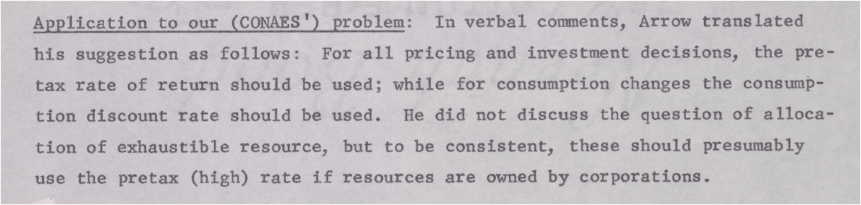
Arrow obliged. He opened his presentation to the group by arguing for the consumer’s utility rate as the theoretical benchmark, over the private market rate. To support this, he solved a Ramsey model, subsequently adding growth and market imperfections, and demonstrated that the riskless rate of return in these models obeyed a Ramsey formula. However, his practical advice did not rely on such theoretical foundation. He proposed a dual discount rate scheme, with a 13% pre-tax rate of return on private investment to calculate the costs of new technologies, and a 6% after-tax return on investment to discount the net benefits of these R&D project on society. He further recommended adjusting these rates to account for project-specific uncertainties. The following week, the team grappled with whether Arrow's suggestions could be extended to allocating exhaustible resources, a challenge he had not addressed.
Arrow thus brought the Ramsey formula to 1970s discounting discussions, but it was then more a theoretical benchmark to convince audiences that the appropriate rate was the social rate for consumption rather than investment. When it came to empirical work, the Ramsey formula then seemed of no use. A similar gap was evident, a few years earlier, when UK growth theorists a familiar with deriving Ramsey formulas from optimal growth models started writing project evaluation guidelines for developing countries, particularly India. Two competing reports came out at the turn of the seventies. One by Mirlees and Ian Little for OECD, the other by Sen, Daguspta and Marglin for the UN. Significant disagreements arose, in particular regarding the adoption of a social discount rate on consumption vs investment. These disagreements reflected underlying conflicting assumptions about the rationality of governments tasked with implementing development projects. The Ramsey formula was nowhere to be found in those debates.

The 1970s, therefore, saw economists involved in energy and growth modeling scratching their head over discounting. But as if juggling formulas and numbers wasn't tricky enough, they didn't just have to argue with one another or with the engineers and scientists they met while writing these massive reports. Perhaps the most daunting part of the job was talking with philosophers.
Next S1E6: “Ramsey does not believe in a time-discount rate bigger than zero; that makes three of us”: ethics strikes back
Homework: guess who were the “three of us”